Wall-models are derived from the averaged governing equations but often applied in practice in an instantaneous sense, i.e., to estimate the instantaneous wall shear stress from the instantaneous velocity at the matching location as \( \tau_{\rm wm}(u; h_{\rm wm}) \) where \( u \) is the instantaneous velocity and \( h_{\rm wm} \) is the thickness of the wall-modeled layer (equivalently, the distance to the exchange location). Note that we are assuming constant density \( \rho \) and viscosity \( \nu \) here, hence those variables are suppressed in the wall-model equation.
Since wall-models are derived from averaged equations and calibrated based on averaged data, the correct mean wall stress is best approximated by \( \tau_{\rm wm}(\overline{u}; h_{\rm wm}) \) where \( \overline{u} \) is the mean velocity. We can then define the relative error in the estimated mean wall stress due to the lack of commutation between averaging and the wall-model as
\begin{equation}\label{eqn:relerror}
E = \frac{
\overline{\tau_{\rm wm}(u; h_{\rm wm})} –
\tau_{\rm wm}(\overline{u}; h_{\rm wm})
}{ \tau_{\rm wm}(\overline{u}; h_{\rm wm}) }
= \frac{ \overline{\tau_{\rm wm}(u; h_{\rm wm})} }{ \overline{\tau}_{w, {\rm correct}} } – 1
\,.
\end{equation}
A Taylor expansion around \( \overline{u} \) yields
\begin{equation}
\overline{\tau_{\rm wm}(u; h_{\rm wm})} \approx
\tau_{\rm wm}(\overline{u}; h_{\rm wm})
+ \frac{1}{2}
\left. \frac{\partial^2 \tau_{\rm wm}}{\partial u^2} \right|_{\overline{u}}
\,
\overline{u’u’}
\,.
\end{equation}
or
\begin{equation}
E \approx
\frac{1}{2 \rho}
\left. \frac{\partial^2 \tau_{\rm wm}}{\partial u^2} \right|_{\overline{u}}
\,
\frac{\rho \overline{u’u’}}{ \overline{\tau}_{w, {\rm correct}} }
\,.
\end{equation}
The relative error is thus proportional to the streamwise Reynolds stress in viscous units with the coefficient of proportionality determined by the second derivative of the model. This second derivative of the wall-model function \( \tau_{\rm wm} (y; h_{\rm wm}) \) must be computed with \( h_{\rm wm} \) fixed in outer units, as done in an actual code. This could be computed numerically for complex wall-models or analytically for simpler ones (using the fact that \( d^2 \tau_{\rm wm}/du^2 = – d^2 u/d\tau_{\rm wm}^2 / (du/d\tau_{\rm wm})^3 \)). The error was computed for Reichardt’s wall-model
\begin{equation}
u^+ = \frac{\ln(1+0.4y^+)}{0.4} + 7.8\left(
1 – e^{-y^+/11} – \frac{y^+}{11} e^{-y^+/3}
\right)
\,.
\end{equation}
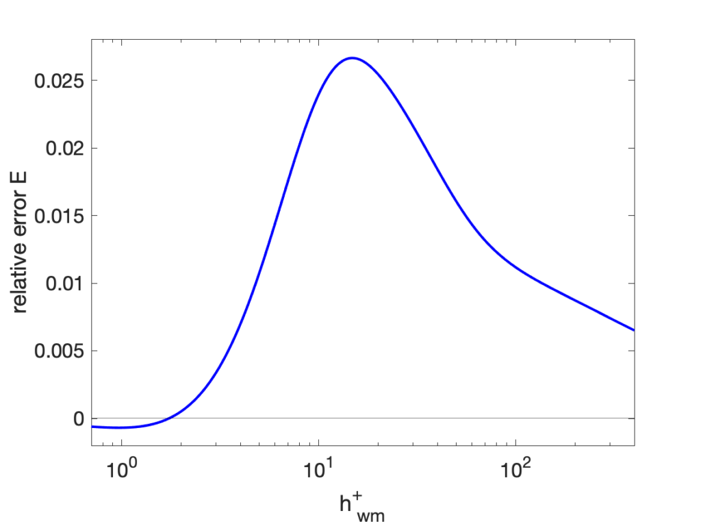
combined with the streamwise Reynolds stress from the DNS data of Sillero et al (2014), with the relative error shown in the figure below. The error peaks at just below 3% in the buffer layer, and decreases towards zero for exchange locations both closer and farther from the wall mainly due to the decreased Reynolds stress. Note that the error is essentially always positive, meaning that the mean wall stress computed by a WMLES will be biased towards larger values when applied instantaneously.

While it is clearly better to supply a wall-model with averaged (or time-filtered, as suggested in parts of the literature) data, the analysis above shows that the error of using instantaneous values is a few percent, which is probably acceptable in most scenarios.