This case was used in the High-Fidelity CFD Verification Workshops organized in 2022 and 2024. The test case was inspired by the experiment of Simmons, Thomas and Corke (AIAA Papers 2017-4128 and 2018-0572), but uses a narrow spanwise periodic domain which prevents direct comparison with the experimental data; therefore, several other aspects of the problem were defined differently from the experiments as well. The 2022 version of the case used a very narrow domain, which was then found to produce unphysical “vortex-shedding-like” structures that made averages converge more slowly. The 2024 version of the case therefore uses a wider (though still narrow enough to affect the results) spanwise domain. The other major change from 2022 to 2024 was that Uzun and Malik (2024) performed a DNS of this problem, which then led to changes in the Reynolds number and thickness of the incoming boundary layer. The description of the problem on this website is the 2024 version of the problem.
Basic set-up
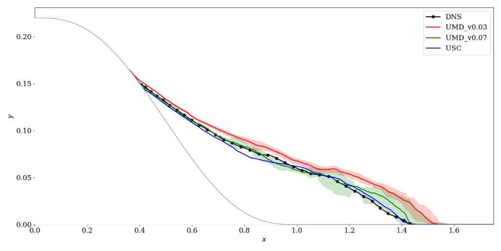
The computational domain is shown in the figure below. The ramp geometry is defined as (Simmons et al, 2017)
\begin{equation} \label{eqn:ramp_geometry}
\frac{y}{L} = 0.22\left[ 1 – 10 \left(\frac{x}{L}\right)^3 + 15 \left(\frac{x}{L}\right)^4 – 6 \left(\frac{x}{L}\right)^5 \right]
\end{equation}
where the ramp begins at \((x,y)=(0,H)\) and \(H/L=0.22\). The top wall is treated as an inviscid wall with slip. The spanwise width of the domain is \(L_z/L=0.288\), with periodic boundary conditions.
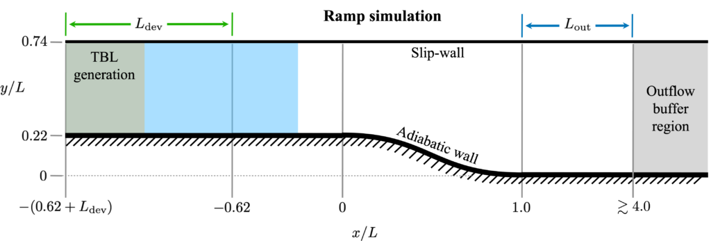
The Reynolds number is \(Re_L=U_\infty L / \nu_\infty=667,000\) where “\(\infty\)” indicates the incoming flow in the potential region. The Mach number is 0.2 at those same conditions. Details of the fluid properties are unlikely to have a strong effect at this low Mach number, and thus the fluid viscosity can be taken as constant.
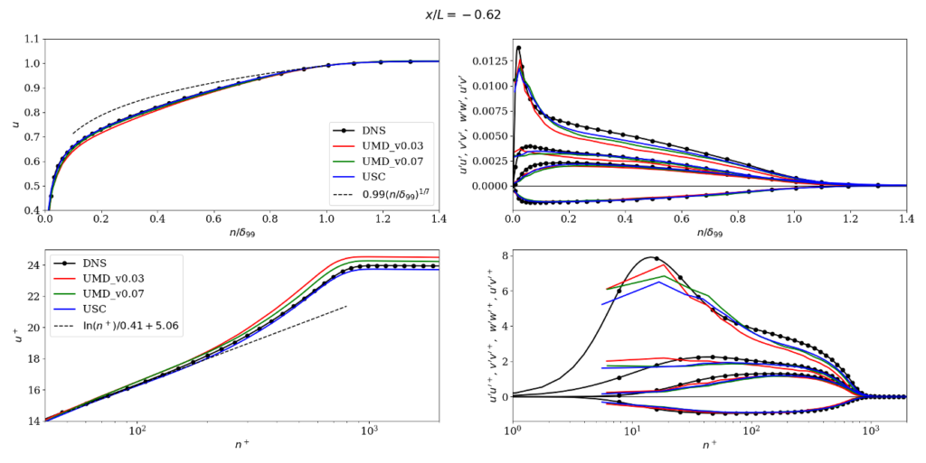
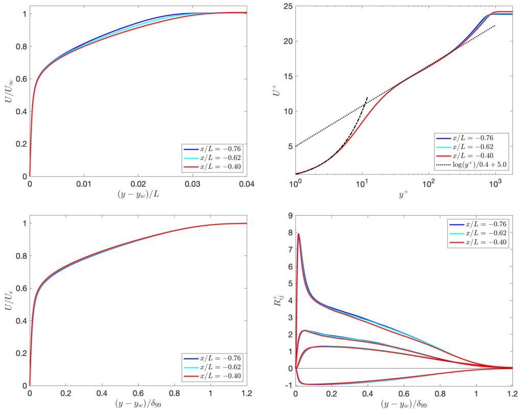
Some type of turbulence generation method is needed at the inflow. The location of the inlet should be chosen to generate a fully developed turbulent boundary layer that matches the DNS as best as possible at the incoming reference locations \(x/L=-0.76, -0.62, -0.40\). Those DNS profiles are shown in the figure below; it is clear that the DNS is fully developed with minimal memory of the inflow condition. The boundary layer thickness is about \(\delta/L\approx 0.028\) at the middle of those locations. The DNS profiles are available here.
The useful part of the domain (where one should strive for accurate results) should extend at least up to \(x/L=4\). Users should then place their outflow and possibly use sponge regions as needed to make sure that the outflow has minimal effect on the flow.
Grids
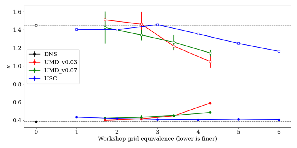
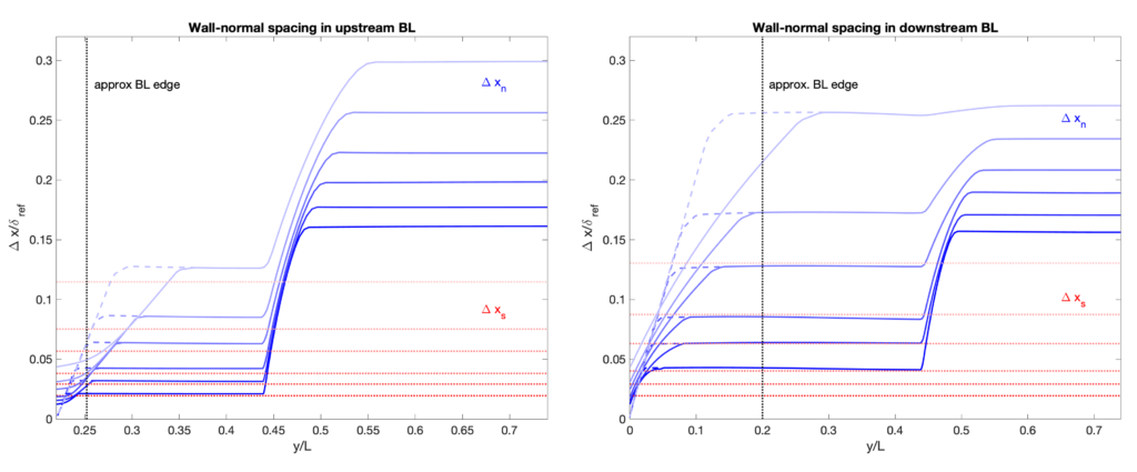
Robert Baurle of NASA Langley generated a whole set of grids for the workshop that are available for download. That directory also contains several ASCII files containing the grid-spacing distributions for those that want to mimic these grids with other grid-generation software. Note that there are 6 levels of refinement, with grid-spacings shown in the figure below. Note that grid 1 is the finest and grid 6 is the coarsest. For submissions that use other grids, an equivalent “grid index” has been estimated based on the cell count (so a “grid 1.7” would have somewhat more cells than the workshop grid 2, for example).
Results
Ivan Bermejo-Moreno from USC created a Python script that automatically creates 20+ different multi-figure plots for each submission (one set of runs on multiple grids) for this case. The following submissions are available at this time:
- The Tortuga::cLes code from the University of Maryland.
- The uPDE code from the University of Southern California.
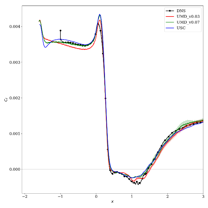
The main comparison between the codes can be found here. Some results are also available in the workshop summary paper by Garmann et al (2024). Some key figures are shown below.