The domain size is taken as \((12.8h, 2h, 4.8h)\), which is smaller than in the DNS by about factors of 2 in the wall-parallel directions. This is done to reduce the computational cost, and will not affect the assessment of the wall-modeling (provided we interpret the results correctly, e.g., accepting differences in the wake region).
The central 80% of the channel constitute the nominal LES region. For wall-stress models, we apply the wall-model over a layer of thickness \(h_{\rm wm}/h = 0.1\). For hybrid LES/RANS models, we place the nominal switch from LES to RANS at the same height.
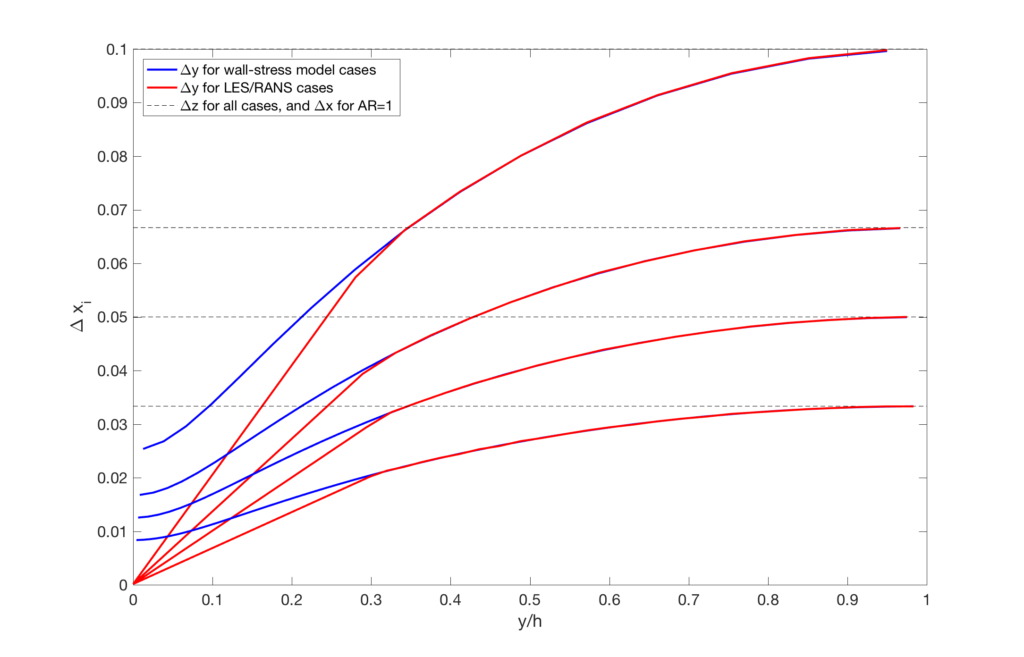
We use grids at 4 different resolution levels in order to judge grid-convergence. The resolution level is quantified (and labeled) by the spanwise resolution \(\Delta z/h\): the 4 grids have \(\Delta z/h =\) 0.100, 0.067, 0.050, and 0.033.
We use grids with 2 different aspect ratios in the wall-parallel plane in order to judge the sensitivity to the grid anisotropy. The base grid has \(\Delta x = \Delta z\) (which is consistent with the idea that one would not know the flow direction a priori for complex flow problems). Given the known sensitivity of LES to grid anisotropy (cf. Meyers and Sagaut, 2007), we also use grids with \(\Delta x = 2\Delta z\). While many (most?) channel flow studies using (WM)LES in the literature used a single \(\Delta x / \Delta z\) ratio and never varied it, it is crucial to appreciate the importance of assessing the sensitivity of a (WM)LES approach to the cell aspect ratio.
There are two versions of every grid: one intended for wall-stress models, one intended for hybrid LES/RANS models. The former have \(\Delta y_w \approx 0.25 \Delta y_c\) (subscripts \(w\) and \(c\) denote the wall and the centerline, respectively) and are refined uniformly and isotropically. The grids for hybrid LES/RANS have \(\Delta y_w / h= 1.5 \! \cdot \! 10^{-4}\) at all resolution levels; this value produces \(\Delta y^+_w \approx 0.8\) which is not refined in order to reduce the time-step penalty for compressible solvers. The wall-stress and hybrid LES/RANS grids have identical grid-spacings in the core 69% of the channel (i.e., for \(y/h \gtrsim 0.31\)). At the centerline, \(\Delta y_c = \Delta z\).
Details on the grids are given in the figure and table below. Note that the number of grid points in the table refers to the vertices (or nodes) — i.e., the number of cells in a finite-volume grid would be one less in each direction.
These grids are made available here in two different ways. For people who want to generate their own grids (e.g., in some research codes), the \(y\)-coordinates for the grids are given in the following ASCII files:
- For wall-stress models: channel_1dwm_33pts, channel_1dwm_49pts, channel_1dwm_65pts, channel_1dwm_97pts.
- For hybrid LES/RANS: channel_intw_77pts, channel_intw_109pts, channel_intw_141pts, channel_intw_197pts.
For people who instead want to use a full grid file (e.g., in a more commercial-like code), the full grids can be created in PLOT3D format in the following way. First, download \(x-y\) slices of the grids in PLOT3D format:
- For wall-stress models, AR=1: channel_ar1_1dwm_129x33, channel_ar1_1dwm_193x49, channel_ar1_1dwm_257x65, channel_ar1_1dwm_385x97.
- For wall-stress models, AR=2: channel_ar2_1dwm_65x33, channel_ar2_1dwm_97x49, channel_ar2_1dwm_129x65, channel_ar2_1dwm_193x97.
- For hybrid LES/RANS, AR=1: channel_ar1_intw_129x77, channel_ar1_intw_193x109, channel_ar1_intw_257x141, channel_ar1_intw_385x197.
- For hybrid LES/RANS, AR=2: channel_ar2_intw_65x77, channel_ar2_intw_97x109, channel_ar2_intw_129x141, channel_ar2_intw_193x197.
These \(x-y\) slices can then be extruded to form the full 3D grid by using the following extrude.f90 code. Currently, the only output format option is PLOT3D (64-bit unformatted). However, the subroutine output_p3d can easily be replaced with a user-defined subroutine to provide grid files in some other format. Note that this utility is set up to produce “double-precision” floating point values by default (as a result the it should NOT be compiled with options to up-convert floating point values, i.e., -r8 is not needed). The extrude.f90 code exports the grid as a PLOT3D unformatted file, i.e., as
  write(unit_num) num_blocks
  write(unit_num) (ni(n), nj(n), nk(n), n=1, num_blocks)
  do n = 1, num_blocks
    write(unit_num)
      ( ( ( x(i,j,k), i=1,ni(n) ) , j=1,nj(n) ) , k=1,nk(n) ) ,
      ( ( ( y(i,j,k), i=1,ni(n) ) , j=1,nj(n) ) , k=1,nk(n) ) ,
      ( ( ( z(i,j,k), i=1,ni(n) ) , j=1,nj(n) ) , k=1,nk(n) )
  end do
but this can easily be modified to output the final 3D grid in other formats. To use this utility, simply compile the fortran source code, e.g.,
\> gfortran -o extrude.out extrude.f90and run the code and answer the prompts.